# solve the elastic double pendulum using fourth order Runge-Kutta method
# Import packages needed
import matplotlib.animation as animation
import timeit
from numpy import sqrt, sin, cos, arange, pi, append, array, floor
from pylab import plot, xlabel, ylabel, title, show, axhline, savefig, subplots_adjust,\
figure, xlim, rcParams, rc, rc_context, subplot, tight_layout, axvline, xlim, ylim, scatter
# get starting time
start = timeit.default_timer()
# define a function to calculate our slopes at a given position
# eta = (theta1, omega1, r1, v1, theta2, omega2, r2, v2)
def f(eta):
theta1 = eta[0]
omega1 = eta[1]
r1 = eta[2]
v1 = eta[3]
theta2 = eta[4]
omega2 = eta[5]
r2 = eta[6]
v2 = eta[7]
f_theta1 = omega1
f_r1 = v1
f_theta2 = omega2
f_r2 = v2
f_omega1 = (k2*(l2-r2)*sin(theta1-theta2) - 2*m1*v1*omega1\
- m1*g*sin(theta1)) / (m1*r1)
f_v1 = (m1*g*cos(theta1) + k1*(l1-r1) - k2*(l2-r2)*cos(theta1-theta2)\
+ m1*r1*omega1**2) / m1
f_omega2 = (-k1*(l1-r1)*sin(theta1-theta2) - 2*m1*v2*omega2) / (m1*r2)
f_v2 = (k2*(m1+m2)*(l2-r2) + m1*m2*r2*omega2**2 -m2*k1*(l1-r1)*cos(theta1-theta2))/(m1*m2)
return(array([f_theta1,f_omega1, f_r1, f_v1, \
f_theta2,f_omega2, f_r2, f_v2],float))
# define a function that takes initial angles and spring compressions in as
# parameters and outputs array of angles and velocities of both masses
def doublePendulumGuy(theta1_initial_deg, theta2_initial_deg, r1_initial, r2_initial):
omega1_initial_deg = 0.0 # initial angular speed
omega2_initial_deg = 0.0 # initial angular speed
theta1_initial = theta1_initial_deg*pi/180 # convert initial angle into degrees
omega1_initial = omega1_initial_deg*pi/180 # convert initial anglular speed into degrees
theta2_initial = theta2_initial_deg*pi/180 # convert initial angle into degrees
omega2_initial = omega2_initial_deg*pi/180 # convert initial anglular speed into degrees
v1_initial = 0.0 # initial value of r1dot
v2_initial = 0.0 # intiial value of r2dot
# set up a domain (time interval of interest)
a = 0.0 # interval start
b = 80.0 # interval end
dt = 0.003 # timestep
t_points = arange(a,b,dt) # array of times
# initial conditions eta = (theta1, omega1, r1, v1, theta2, omega2, r2, v2)
eta = array([theta1_initial, omega1_initial, r1_initial, v1_initial, \
theta2_initial, omega2_initial, r2_initial, v2_initial],float)
# create empty sets to update with values of interest, then invoke Runge-Kutta
theta1_points = []
omega1_points = []
r1_points = []
v1_points = []
theta2_points = []
omega2_points = []
r2_points = []
v2_points = []
energy_points = []
for t in t_points:
theta1_points.append(eta[0])
omega1_points.append(eta[1])
r1_points.append(eta[2])
v1_points.append(eta[3])
theta2_points.append(eta[4])
omega2_points.append(eta[5])
r2_points.append(eta[6])
v2_points.append(eta[7])
E_1 = 0.5*m1*(eta[3]**2 + eta[2]**2 * eta[1]**2) + 0.5*k1*(l1-eta[2])**2 \
- m1*g*eta[2]*cos(eta[0])
E_2 = 0.5*m2*(eta[3]**2 + eta[7]**2) + m2*(-sin(eta[0]-eta[4])*eta[2]*eta[7]*eta[1] \
+ eta[2]**2 * eta[1]**2 + cos(eta[0]-eta[4])*eta[2]*eta[6]*eta[1]*eta[5] \
+ 0.5*eta[6]**2 * eta[5]**2 + eta[3]*(cos(eta[0]-eta[4])*eta[7] \
+ sin(eta[0]-eta[4])*eta[6]*eta[5])) + 0.5*k2*(l2-eta[6])**2 \
- m2*g*(cos(eta[0])*eta[2] + cos(eta[4])*eta[6])
E_net = E_1 + E_2
energy_points.append(E_net)
kutta1 = dt*f(eta)
kutta2 = dt*f(eta + 0.5*kutta1)
kutta3 = dt*f(eta + 0.5*kutta2)
kutta4 = dt*f(eta + kutta3)
eta += (kutta1 + 2*kutta2 + 2*kutta3 + kutta4)/6
return(theta1_points, omega1_points, r1_points, v1_points, \
theta2_points, omega2_points, r2_points, v2_points, t_points, energy_points)
# set up the parameters of our situation
m1 = 5.00 # mass of bob 1
m2 = 3.50 # mass of bob 2
l1 = 0.85 # equilibrium length of spring 1
l2 = 1.20 # equilibrium length of spring 2
k1 = 80.0 # spring constant for spring 1
k2 = 90.0 # spring constant for spring 2
g = 9.81 # acceleration due to gravity
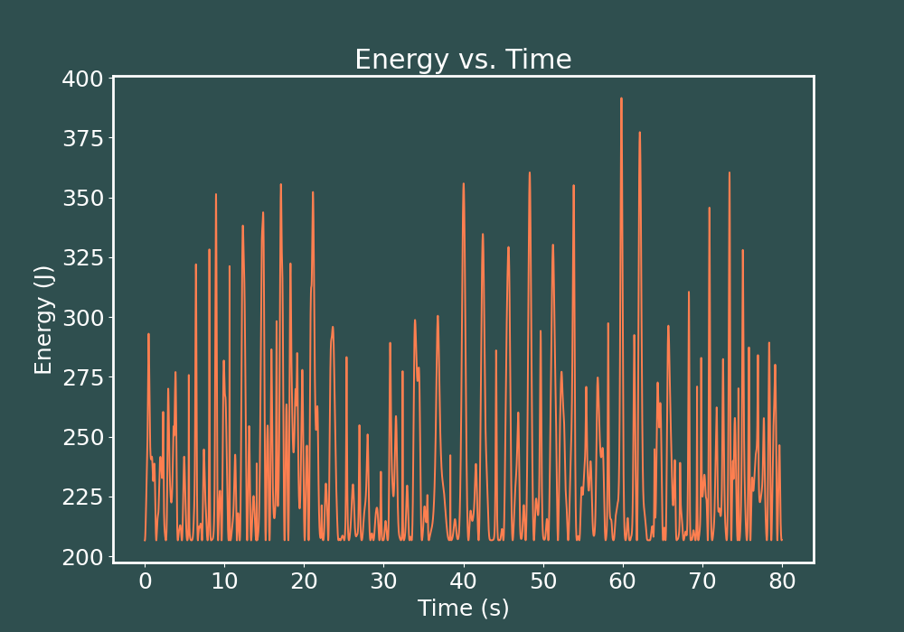
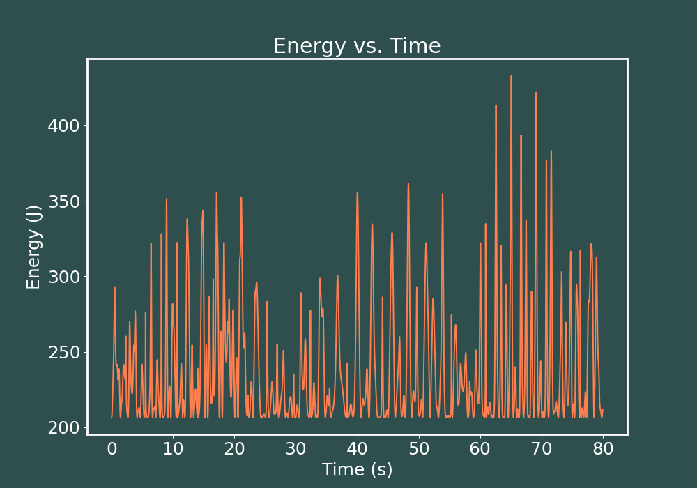
# call the function and store the arrays of data
theta1_points, omega1_points, r1_points, v1_points, theta2_points, omega2_points,\
r2_points, v2_points, t_points, energy_points = doublePendulumGuy(170,105, l1*1.65, l2*1.95)
# create lists of x and y values for bob1 and 2
x1_points = []
y1_points = []
x2_points = []
y2_points = []
for i in range(len(t_points)):
x1_new = r1_points[i]*sin(theta1_points[i])
y1_new = -r1_points[i]*cos(theta1_points[i])
x1_points.append(x1_new)
y1_points.append(y1_new)
x2_new = r1_points[i]*sin(theta1_points[i]) + r2_points[i]*sin(theta2_points[i])
y2_new = -r1_points[i]*cos(theta1_points[i]) - r2_points[i]*cos(theta2_points[i])
x2_points.append(x2_new)
y2_points.append(y2_new)
# animate our results
# start with styling options
rcParams.update({'font.size': 18})
rc('axes', linewidth=2)
with rc_context({'axes.edgecolor':'white', 'xtick.color':'white', \
'ytick.color':'white', 'figure.facecolor':'darkslategrey',\
'axes.facecolor':'darkslategrey','axes.labelcolor':'white',\
'axes.titlecolor':'white'}):
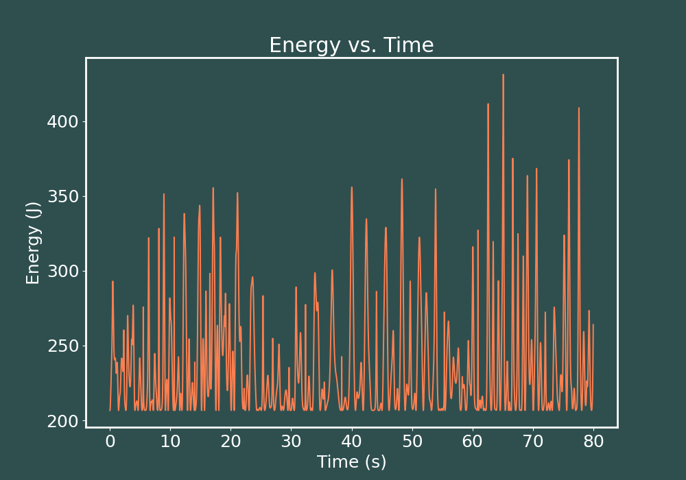
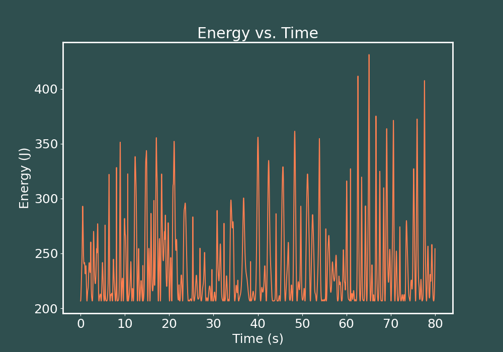
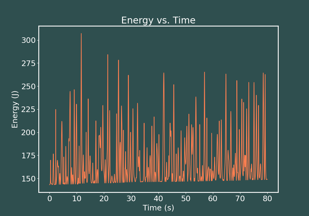
# subplot for the graph of energy vs time
fig_E = figure(figsize=(10,7))
ax_energy = subplot(1,1,1)
title("Energy vs. Time")
xlabel("Time (s)")
ylabel("Energy (J)")
ax_energy.plot(t_points,energy_points,color='coral',lw=1.4)
savefig("../elasticDoublePendulum/175_185_elasticDoublePend_energy_kutta003.png")
# print runtime of our code
stop = timeit.default_timer()
print('Time: ', stop - start)
# set up a figure for pendulum
fig = figure(figsize=(10,10))
# subplot for animation of pendulum
ax_pend = subplot(1,1,1, aspect='equal')
# get rid of axis ticks
ax_pend.tick_params(axis='both', colors="darkslategrey")
### finally we animate ###
# create a list to input images in for each time step
ims = []
index = 0
# only show the first 80seconds or so in the gif
while index <= len(t_points)-1:
ln1, = ax_pend.plot([0,r1_points[index]*sin(theta1_points[index])],\
[0,-r1_points[index]*cos(theta1_points[index])],\
color='k',lw=3,zorder=99)
bob1, = ax_pend.plot(r1_points[index]*sin(theta1_points[index]),\
-r1_points[index]*cos(theta1_points[index]),'o',\
markersize=22,color="m",zorder=100)
ln2, = ax_pend.plot([r1_points[index]*sin(theta1_points[index]),\
r1_points[index]*sin(theta1_points[index])+\
r2_points[index]*sin(theta2_points[index])],\
[-r1_points[index]*cos(theta1_points[index]),\
-r1_points[index]*cos(theta1_points[index])\
-r2_points[index]*cos(theta2_points[index])], color='k',lw=3,zorder=99)
bob2, = ax_pend.plot(r1_points[index]*sin(theta1_points[index])+\
r2_points[index]*sin(theta2_points[index]),\
-r1_points[index]*cos(theta1_points[index])\
-r2_points[index]*cos(theta2_points[index]),'o',\
markersize=22,color="coral",zorder=100)
if index > 200:
trail1, = ax_pend.plot(x1_points[index-140:index],y1_points[index-140:index], \
color="lime",lw=0.8,zorder=20)
trail2, = ax_pend.plot(x2_points[index-190:index],y2_points[index-190:index], \
color="cyan",lw=0.8,zorder=20)
else:
trail1, = ax_pend.plot(x1_points[:index],y1_points[:index], \
color="lime",lw=0.8,zorder=20)
trail2, = ax_pend.plot(x2_points[:index],y2_points[:index], \
color="cyan",lw=0.8,zorder=20)
# add pictures to ims list
ims.append([ln1, bob1, ln2, bob2, trail1, trail2])
# only show every 6 frames
index += 6
# save animations
ani = animation.ArtistAnimation(fig, ims, interval=100)
writervideo = animation.FFMpegWriter(fps=60)
ani.save('../elasticDoublePendulum/170_105_elasticDoublePend.mp4', writer=writervideo)
# solve the elastic pendulum using fourth order Runge-Kutta method
# Import packages needed
import matplotlib.animation as animation
import timeit
from numpy import sqrt, sin, cos, arange, pi, append, array, floor
from pylab import plot, xlabel, ylabel, title, show, axhline, savefig, subplots_adjust,\
figure, xlim, rcParams, rc, rc_context, subplot, tight_layout, axvline, xlim, ylim, scatter
# start get starting time
start = timeit.default_timer()
# define a function that takes initial angles and spring compressions in as
# parameters and outputs array of angles and velocities of both masses
def doublePendulumGuy(theta1_initial_deg, theta2_initial_deg, r1_initial, r2_initial):
omega1_initial_deg = 0.0 # initial angular speed
omega2_initial_deg = 0.0 # initial angular speed
theta1_c = theta1_initial_deg*pi/180 # convert initial angle into degrees
omega1_c = omega1_initial_deg*pi/180 # convert initial anglular speed into degrees
theta2_c = theta2_initial_deg*pi/180 # convert initial angle into degrees
omega2_c = omega2_initial_deg*pi/180 # convert initial anglular speed into degrees
r1_c = r1_initial # initial length of spring 1
r2_c = r2_initial # initial length of spring 2
v1_c = 0.0 # initial value of r1dot
v2_c = 0.0 # intiial value of r2dot
# set up a domain (time interval of interest)
a = 0.0 # interval start
b = 60.0 # interval end
dt = 0.002 # timestep
t_points = arange(a,b,dt) # array of times
# create empty sets to update with values of interest, then invoke Euler-Cromer
energy_points = []
for t in t_points:
# find the net energy this step
E_1 = 0.5*m1*(v1_c**2 + r1_c**2 * omega1_c**2) + 0.5*k1*(l1-r1_c)**2 \
- m1*g*r1_c*cos(theta1_c)
E_2 = 0.5*m2*(v1_c**2 + v2_c**2) + m2*(-sin(theta1_c-theta2_c)*r1_c*v2_c*omega1_c \
+ r1_c**2 * omega1_c**2 + cos(theta1_c-theta2_c)*r1_c*r2_c*omega1_c*omega2_c \
+ 0.5*r2_c**2 * omega2_c**2 + v1_c*(cos(theta1_c-theta2_c)*v2_c \
+ sin(theta1_c-theta2_c)*r2_c*omega2_c)) + 0.5*k2*(l2-r2_c)**2 \
- m2*g*(cos(theta1_c)*r1_c + cos(theta2_c)*r2_c)
E_net = E_1 + E_2
energy_points.append(E_net)
# define slopes of velocities at this step
f_omega1 = (-4*sin(theta1_c-theta2_c) + k2*(l2-r2_c)*sin(theta1_c-theta2_c) - 2*m1*v1_c*omega1_c\
- m1*g*sin(theta1_c)) / (m1*r1_c)
f_v1 = (4*cos(theta1_c-theta2_c) + m1*g*cos(theta1_c) + k1*(l1-r1_c) \
- k2*(l2-r2_c)*cos(theta1_c-theta2_c) + m1*r1_c*omega1_c**2) / m1
f_omega2 = (-k1*(l1-r1_c)*sin(theta1_c-theta2_c) - 2*m1*v2_c*omega2_c) / (m1*r2_c)
f_v2 = (k2*(l2-r2_c) - k1*(l1-r1_c)*cos(theta1_c-theta2_c) - 4) / m1 \
+ (k2*(l2-r2_c) + m2*r2_c*omega2_c**2) / m2
# caculate next velocities (i+1) using current values
omega1_n = omega1_c + dt*f_omega1
v1_n = v1_c + dt*f_v1
omega2_n = omega2_c + dt*f_omega2
v2_n = v2_c + dt*f_v2
# now we define the slopes of our positions using the values of
# velocities in the next step
f_theta1 = omega1_n
f_r1 = v1_n
f_theta2 = omega2_n
f_r2 = v2_n
# find our new positions (i+1) using the velocities at (i+1)
theta1_n = theta1_c + dt*f_theta1
r1_n = r1_c + dt*f_r1
theta2_n = theta2_c + dt*f_theta2
r2_n = r2_c + dt*f_r2
# update current conditions
theta1_c = theta1_n
omega1_c = omega1_n
r1_c = r1_n
v1_c = v1_n
theta2_c = theta2_n
omega2_c = omega2_n
r2_c = r2_n
v2_c = v2_n
return(t_points, energy_points)
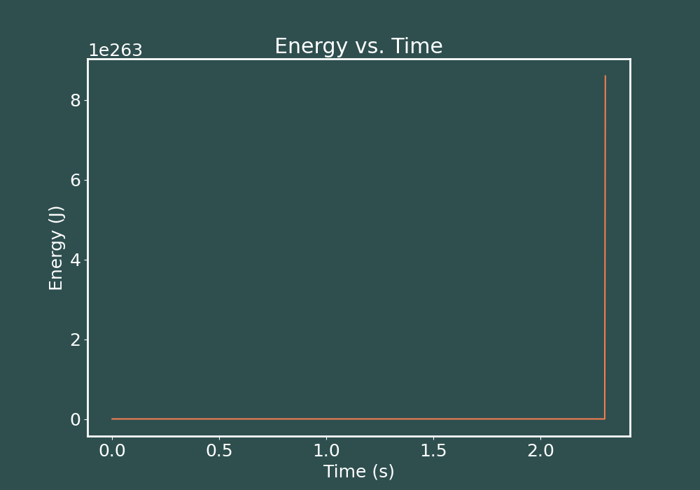
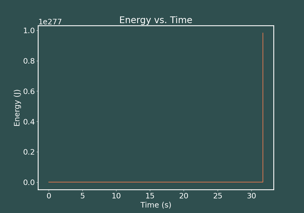
# set up the parameters of our situation
m1 = 5.00 # mass of bob 1
m2 = 3.50 # mass of bob 2
l1 = 0.85 # equilibrium length of spring 1
l2 = 1.20 # equilibrium length of spring 2
k1 = 80.0 # spring constant for spring 1
k2 = 90.0 # spring constant for spring 2
g = 9.81 # acceleration due to gravity
# call the function and store the arrays of data
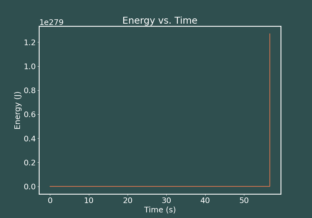
t_points, energy_points = doublePendulumGuy(175,185, l1*1.45, l2*0.6)
# Create our energy vs. time graoh
# start with styling options
rcParams.update({'font.size': 18})
rc('axes', linewidth=2)
with rc_context({'axes.edgecolor':'white', 'xtick.color':'white', \
'ytick.color':'white', 'figure.facecolor':'darkslategrey',\
'axes.facecolor':'darkslategrey','axes.labelcolor':'white',\
'axes.titlecolor':'white'}):
# subplot for the graph of energy vs time
fig_E = figure(figsize=(10,7))
ax_energy = subplot(1,1,1)
title("Energy vs. Time")
xlabel("Time (s)")
ylabel("Energy (J)")
ax_energy.plot(t_points,energy_points,color='coral',lw=1.4)
savefig("../elasticDoublePendulum/175_185_elasticDoublePend_energy_euler-cromer002.png")
# print time it took our code to run
stop = timeit.default_timer()
print('Time: ', stop - start)